Augmentation#
Augmentation transforms generate different results every time they are called.
Base class#
RandomTransform#
Composition#
Compose#
OneOf#
- class torchio.transforms.OneOf(transforms: Dict[Transform, float] | Sequence[Transform], **kwargs)[source]#
Bases:
RandomTransformApply only one of the given transforms.
- Parameters:
Example
>>> import torchio as tio
>>> colin = tio.datasets.Colin27()
>>> transforms_dict = {
...     tio.RandomAffine(): 0.75,
...     tio.RandomElasticDeformation(): 0.25,
... }  # Using 3 and 1 as probabilities would have the same effect
>>> transform = tio.OneOf(transforms_dict)
>>> transformed = transform(colin)
Spatial#
RandomFlip#
- class torchio.transforms.RandomFlip(axes: int | Tuple[int, ...] = 0, flip_probability: float = 0.5, **kwargs)[source]#
Bases:
RandomTransform,SpatialTransformReverse the order of elements in an image along the given axes.
- Parameters:
axes – Index or tuple of indices of the spatial dimensions along which the image might be flipped. If they are integers, they must be in
(0, 1, 2). Anatomical labels may also be used, such as'Left','Right','Anterior','Posterior','Inferior','Superior','Height'and'Width','AP'(antero-posterior),'lr'(lateral),'w'(width) or'i'(inferior). Only the first letter of the string will be used. If the image is 2D,'Height'and'Width'may be used.flip_probability – Probability that the image will be flipped. This is computed on a per-axis basis.
**kwargs – See
Transformfor additional keyword arguments.
Example
>>> import torchio as tio
>>> fpg = tio.datasets.FPG()
>>> flip = tio.RandomFlip(axes=('LR',))  # flip along lateral axis only
Tip
It is handy to specify the axes as anatomical labels when the image orientation is not known.
RandomAffine#
- class torchio.transforms.RandomAffine(scales: float | Tuple[float, float] | Tuple[float, float, float] | Tuple[float, float, float, float, float, float] = 0.1, degrees: float | Tuple[float, float] | Tuple[float, float, float] | Tuple[float, float, float, float, float, float] = 10, translation: float | Tuple[float, float] | Tuple[float, float, float] | Tuple[float, float, float, float, float, float] = 0, isotropic: bool = False, center: str = 'image', default_pad_value: str | float = 'minimum', image_interpolation: str = 'linear', label_interpolation: str = 'nearest', check_shape: bool = True, **kwargs)[source]#
Bases:
RandomTransform,SpatialTransformApply a random affine transformation and resample the image.
- Parameters:
scales – Tuple \((a_1, b_1, a_2, b_2, a_3, b_3)\) defining the scaling ranges. The scaling values along each dimension are \((s_1, s_2, s_3)\), where \(s_i \sim \mathcal{U}(a_i, b_i)\). If two values \((a, b)\) are provided, then \(s_i \sim \mathcal{U}(a, b)\). If only one value \(x\) is provided, then \(s_i \sim \mathcal{U}(1 - x, 1 + x)\). If three values \((x_1, x_2, x_3)\) are provided, then \(s_i \sim \mathcal{U}(1 - x_i, 1 + x_i)\). For example, using
scales=(0.5, 0.5)will zoom out the image, making the objects inside look twice as small while preserving the physical size and position of the image bounds.degrees – Tuple \((a_1, b_1, a_2, b_2, a_3, b_3)\) defining the rotation ranges in degrees. Rotation angles around each axis are \((\theta_1, \theta_2, \theta_3)\), where \(\theta_i \sim \mathcal{U}(a_i, b_i)\). If two values \((a, b)\) are provided, then \(\theta_i \sim \mathcal{U}(a, b)\). If only one value \(x\) is provided, then \(\theta_i \sim \mathcal{U}(-x, x)\). If three values \((x_1, x_2, x_3)\) are provided, then \(\theta_i \sim \mathcal{U}(-x_i, x_i)\).
translation – Tuple \((a_1, b_1, a_2, b_2, a_3, b_3)\) defining the translation ranges in mm. Translation along each axis is \((t_1, t_2, t_3)\), where \(t_i \sim \mathcal{U}(a_i, b_i)\). If two values \((a, b)\) are provided, then \(t_i \sim \mathcal{U}(a, b)\). If only one value \(x\) is provided, then \(t_i \sim \mathcal{U}(-x, x)\). If three values \((x_1, x_2, x_3)\) are provided, then \(t_i \sim \mathcal{U}(-x_i, x_i)\). For example, if the image is in RAS+ orientation (e.g., after applying
ToCanonical) and the translation is \((10, 20, 30)\), the sample will move 10 mm to the right, 20 mm to the front, and 30 mm upwards. If the image was in, e.g., PIR+ orientation, the sample will move 10 mm to the back, 20 mm downwards, and 30 mm to the right.isotropic – If
True, the scaling factor along all dimensions is the same, i.e. \(s_1 = s_2 = s_3\).center – If
'image', rotations and scaling will be performed around the image center. If'origin', rotations and scaling will be performed around the origin in world coordinates.default_pad_value – As the image is rotated, some values near the borders will be undefined. If
'minimum', the fill value will be the image minimum. If'mean', the fill value is the mean of the border values. If'otsu', the fill value is the mean of the values at the border that lie under an Otsu threshold. If it is a number, that value will be used.image_interpolation – See Interpolation.
label_interpolation – See Interpolation.
check_shape – If
Truean error will be raised if the images are in different physical spaces. IfFalse,centershould probably not be'image'but'center'.**kwargs – See
Transformfor additional keyword arguments.
Example
>>> import torchio as tio
>>> image = tio.datasets.Colin27().t1
>>> transform = tio.RandomAffine(
...     scales=(0.9, 1.2),
...     degrees=15,
... )
>>> transformed = transform(image)
(
Source code,png)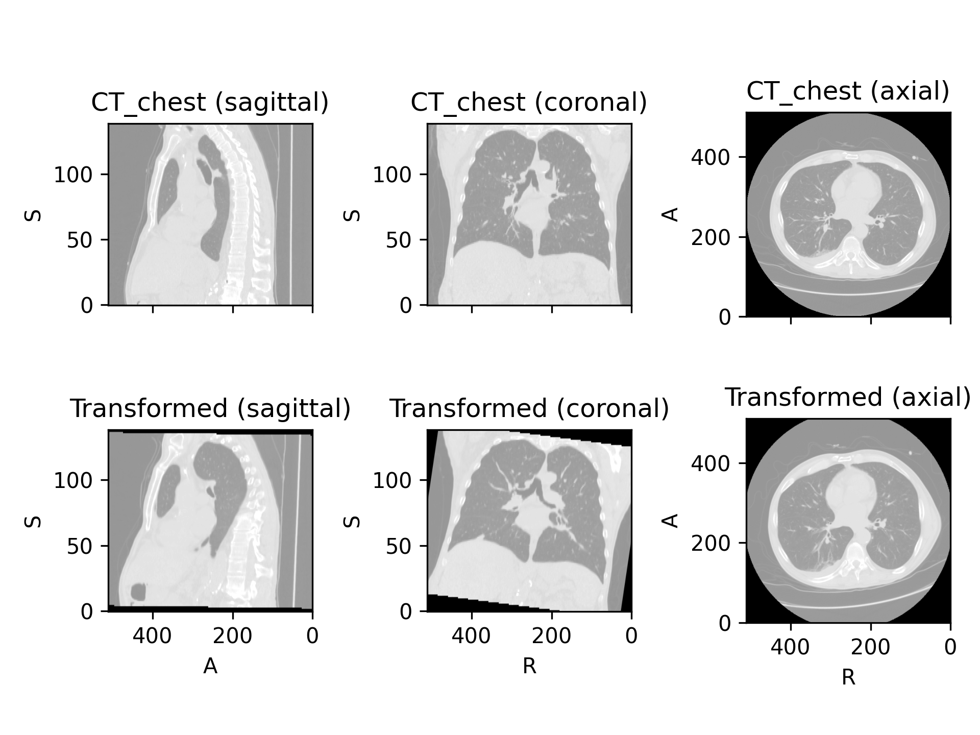
RandomElasticDeformation#
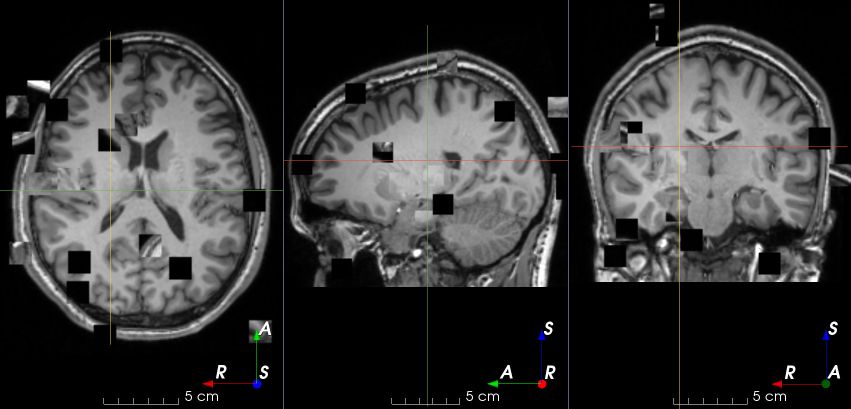
- class torchio.transforms.RandomElasticDeformation(num_control_points: int | Tuple[int, int, int] = 7, max_displacement: float | Tuple[float, float, float] = 7.5, locked_borders: int = 2, image_interpolation: str = 'linear', label_interpolation: str = 'nearest', **kwargs)[source]#
Bases:
RandomTransform,SpatialTransformApply dense random elastic deformation.
A random displacement is assigned to a coarse grid of control points around and inside the image. The displacement at each voxel is interpolated from the coarse grid using cubic B-splines.
The ‘Deformable Registration’ topic on ScienceDirect contains useful articles explaining interpolation of displacement fields using cubic B-splines.
Warning
This transform is slow as it requires expensive computations. If your images are large you might want to use
RandomAffineinstead.- Parameters:
num_control_points – Number of control points along each dimension of the coarse grid \((n_x, n_y, n_z)\). If a single value \(n\) is passed, then \(n_x = n_y = n_z = n\). Smaller numbers generate smoother deformations. The minimum number of control points is
4as this transform uses cubic B-splines to interpolate displacement.max_displacement – Maximum displacement along each dimension at each control point \((D_x, D_y, D_z)\). The displacement along dimension \(i\) at each control point is \(d_i \sim \mathcal{U}(0, D_i)\). If a single value \(D\) is passed, then \(D_x = D_y = D_z = D\). Note that the total maximum displacement would actually be \(D_{max} = \sqrt{D_x^2 + D_y^2 + D_z^2}\).
locked_borders – If
0, all displacement vectors are kept. If1, displacement of control points at the border of the coarse grid will be set to0. If2, displacement of control points at the border of the image (red dots in the image below) will also be set to0.image_interpolation – See Interpolation. Note that this is the interpolation used to compute voxel intensities when resampling using the dense displacement field. The value of the dense displacement at each voxel is always interpolated with cubic B-splines from the values at the control points of the coarse grid.
label_interpolation – See Interpolation.
**kwargs – See
Transformfor additional keyword arguments.
This gist can also be used to better understand the meaning of the parameters.
This is an example from the 3D Slicer registration FAQ.
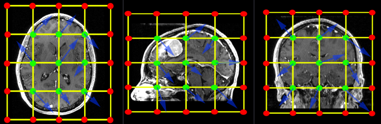
To generate a similar grid of control points with TorchIO, the transform can be instantiated as follows:
>>> from torchio import RandomElasticDeformation
>>> transform = RandomElasticDeformation(
...     num_control_points=(7, 7, 7),  # or just 7
...     locked_borders=2,
... )
Note that control points outside the image bounds are not showed in the example image (they would also be red as we set
locked_bordersto2).Warning
Image folding may occur if the maximum displacement is larger than half the coarse grid spacing. The grid spacing can be computed using the image bounds in physical space [1] and the number of control points:
>>> import numpy as np
>>> import torchio as tio
>>> image = tio.datasets.Slicer().MRHead.as_sitk()
>>> image.GetSize()  # in voxels
(256, 256, 130)
>>> image.GetSpacing()  # in mm
(1.0, 1.0, 1.2999954223632812)
>>> bounds = np.array(image.GetSize()) * np.array(image.GetSpacing())
>>> bounds  # mm
array([256.        , 256.        , 168.99940491])
>>> num_control_points = np.array((7, 7, 6))
>>> grid_spacing = bounds / (num_control_points - 2)
>>> grid_spacing
array([51.2       , 51.2       , 42.24985123])
>>> potential_folding = grid_spacing / 2
>>> potential_folding  # mm
array([25.6       , 25.6       , 21.12492561])
Using a
max_displacementlarger than the computedpotential_foldingwill raise aRuntimeWarning.
RandomAnisotropy#
- class torchio.transforms.RandomAnisotropy(axes: int | Tuple[int, ...] = (0, 1, 2), downsampling: float | Tuple[float, float] = (1.5, 5), image_interpolation: str = 'linear', scalars_only: bool = True, **kwargs)[source]#
Bases:
RandomTransformDownsample an image along an axis and upsample to initial space.
This transform simulates an image that has been acquired using anisotropic spacing and resampled back to its original spacing.
Similar to the work by Billot et al.: Partial Volume Segmentation of Brain MRI Scans of any Resolution and Contrast.
- Parameters:
axes – Axis or tuple of axes along which the image will be downsampled.
downsampling – Downsampling factor \(m \gt 1\). If a tuple \((a, b)\) is provided then \(m \sim \mathcal{U}(a, b)\).
image_interpolation – Image interpolation used to upsample the image back to its initial spacing. Downsampling is performed using nearest neighbor interpolation. See Interpolation for supported interpolation types.
scalars_only – Apply only to instances of
torchio.ScalarImage. This is useful when the segmentation quality needs to be kept, as in Billot et al..**kwargs – See
Transformfor additional keyword arguments.
Example
>>> import torchio as tio
>>> transform = tio.RandomAnisotropy(axes=1, downsampling=2)
>>> transform = tio.RandomAnisotropy(
...     axes=(0, 1, 2),
...     downsampling=(2, 5),
... )   # Multiply spacing of one of the 3 axes by a factor randomly chosen in [2, 5]
>>> colin = tio.datasets.Colin27()
>>> transformed = transform(colin)
Intensity#
RandomMotion#
- class torchio.transforms.RandomMotion(degrees: float | Tuple[float, float] = 10, translation: float | Tuple[float, float] = 10, num_transforms: int = 2, image_interpolation: str = 'linear', **kwargs)[source]#
Bases:
RandomTransform,IntensityTransform,FourierTransformAdd random MRI motion artifact.
Magnetic resonance images suffer from motion artifacts when the subject moves during image acquisition. This transform follows Shaw et al., 2019 to simulate motion artifacts for data augmentation.
- Parameters:
degrees – Tuple \((a, b)\) defining the rotation range in degrees of the simulated movements. The rotation angles around each axis are \((\theta_1, \theta_2, \theta_3)\), where \(\theta_i \sim \mathcal{U}(a, b)\). If only one value \(d\) is provided, \(\theta_i \sim \mathcal{U}(-d, d)\). Larger values generate more distorted images.
translation – Tuple \((a, b)\) defining the translation in mm of the simulated movements. The translations along each axis are \((t_1, t_2, t_3)\), where \(t_i \sim \mathcal{U}(a, b)\). If only one value \(t\) is provided, \(t_i \sim \mathcal{U}(-t, t)\). Larger values generate more distorted images.
num_transforms – Number of simulated movements. Larger values generate more distorted images.
image_interpolation – See Interpolation.
**kwargs – See
Transformfor additional keyword arguments.
Warning
Large numbers of movements lead to longer execution times for 3D images.
RandomGhosting#
- class torchio.transforms.RandomGhosting(num_ghosts: int | Tuple[int, int] = (4, 10), axes: int | Tuple[int, ...] = (0, 1, 2), intensity: float | Tuple[float, float] = (0.5, 1), restore: float = 0.02, **kwargs)[source]#
Bases:
RandomTransform,IntensityTransformAdd random MRI ghosting artifact.
Discrete “ghost” artifacts may occur along the phase-encode direction whenever the position or signal intensity of imaged structures within the field-of-view vary or move in a regular (periodic) fashion. Pulsatile flow of blood or CSF, cardiac motion, and respiratory motion are the most important patient-related causes of ghost artifacts in clinical MR imaging (from mriquestions.com).
- Parameters:
num_ghosts – Number of ‘ghosts’ \(n\) in the image. If
num_ghostsis a tuple \((a, b)\), then \(n \sim \mathcal{U}(a, b) \cap \mathbb{N}\). If only one value \(d\) is provided, \(n \sim \mathcal{U}(0, d) \cap \mathbb{N}\).axes – Axis along which the ghosts will be created. If
axesis a tuple, the axis will be randomly chosen from the passed values. Anatomical labels may also be used (seeRandomFlip).intensity – Positive number representing the artifact strength \(s\) with respect to the maximum of the \(k\)-space. If
0, the ghosts will not be visible. If a tuple \((a, b)\) is provided then \(s \sim \mathcal{U}(a, b)\). If only one value \(d\) is provided, \(s \sim \mathcal{U}(0, d)\).restore – Number between
0and1indicating how much of the \(k\)-space center should be restored after removing the planes that generate the artifact.**kwargs – See
Transformfor additional keyword arguments.
Note
The execution time of this transform does not depend on the number of ghosts.
RandomSpike#
- class torchio.transforms.RandomSpike(num_spikes: int | Tuple[int, int] = 1, intensity: float | Tuple[float, float] = (1, 3), **kwargs)[source]#
Bases:
RandomTransform,IntensityTransform,FourierTransformAdd random MRI spike artifacts.
Also known as Herringbone artifact, crisscross artifact or corduroy artifact, it creates stripes in different directions in image space due to spikes in k-space.
- Parameters:
num_spikes – Number of spikes \(n\) present in k-space. If a tuple \((a, b)\) is provided, then \(n \sim \mathcal{U}(a, b) \cap \mathbb{N}\). If only one value \(d\) is provided, \(n \sim \mathcal{U}(0, d) \cap \mathbb{N}\). Larger values generate more distorted images.
intensity – Ratio \(r\) between the spike intensity and the maximum of the spectrum. If a tuple \((a, b)\) is provided, then \(r \sim \mathcal{U}(a, b)\). If only one value \(d\) is provided, \(r \sim \mathcal{U}(-d, d)\). Larger values generate more distorted images.
**kwargs – See
Transformfor additional keyword arguments.
Note
The execution time of this transform does not depend on the number of spikes.
RandomBiasField#

- class torchio.transforms.RandomBiasField(coefficients: float | Tuple[float, float] = 0.5, order: int = 3, **kwargs)[source]#
Bases:
RandomTransform,IntensityTransformAdd random MRI bias field artifact.
MRI magnetic field inhomogeneity creates intensity variations of very low frequency across the whole image.
The bias field is modeled as a linear combination of polynomial basis functions, as in K. Van Leemput et al., 1999, Automated model-based tissue classification of MR images of the brain.
It was implemented in NiftyNet by Carole Sudre and used in Sudre et al., 2017, Longitudinal segmentation of age-related white matter hyperintensities.
- Parameters:
coefficients – Maximum magnitude \(n\) of polynomial coefficients. If a tuple \((a, b)\) is specified, then \(n \sim \mathcal{U}(a, b)\).
order – Order of the basis polynomial functions.
**kwargs – See
Transformfor additional keyword arguments.
RandomBlur#
- class torchio.transforms.RandomBlur(std: float | Tuple[float, float] = (0, 2), **kwargs)[source]#
Bases:
RandomTransform,IntensityTransformBlur an image using a random-sized Gaussian filter.
- Parameters:
std – Tuple \((a_1, b_1, a_2, b_2, a_3, b_3)\) representing the ranges (in mm) of the standard deviations \((\sigma_1, \sigma_2, \sigma_3)\) of the Gaussian kernels used to blur the image along each axis, where \(\sigma_i \sim \mathcal{U}(a_i, b_i)\). If two values \((a, b)\) are provided, then \(\sigma_i \sim \mathcal{U}(a, b)\). If only one value \(x\) is provided, then \(\sigma_i \sim \mathcal{U}(0, x)\). If three values \((x_1, x_2, x_3)\) are provided, then \(\sigma_i \sim \mathcal{U}(0, x_i)\).
**kwargs – See
Transformfor additional keyword arguments.
RandomNoise#
- class torchio.transforms.RandomNoise(mean: float | Tuple[float, float] = 0, std: float | Tuple[float, float] = (0, 0.25), **kwargs)[source]#
Bases:
RandomTransform,IntensityTransformAdd Gaussian noise with random parameters.
Add noise sampled from a normal distribution with random parameters.
- Parameters:
mean – Mean \(\mu\) of the Gaussian distribution from which the noise is sampled. If two values \((a, b)\) are provided, then \(\mu \sim \mathcal{U}(a, b)\). If only one value \(d\) is provided, \(\mu \sim \mathcal{U}(-d, d)\).
std – Standard deviation \(\sigma\) of the Gaussian distribution from which the noise is sampled. If two values \((a, b)\) are provided, then \(\sigma \sim \mathcal{U}(a, b)\). If only one value \(d\) is provided, \(\sigma \sim \mathcal{U}(0, d)\).
**kwargs – See
Transformfor additional keyword arguments.
RandomSwap#
- class torchio.transforms.RandomSwap(patch_size: int | Tuple[int, int, int] = 15, num_iterations: int = 100, **kwargs)[source]#
Bases:
RandomTransform,IntensityTransformRandomly swap patches within an image.
This is typically used in context restoration for self-supervised learning.
- Parameters:
patch_size – Tuple of integers \((w, h, d)\) to swap patches of size \(w \times h \times d\). If a single number \(n\) is provided, \(w = h = d = n\).
num_iterations – Number of times that two patches will be swapped.
**kwargs – See
Transformfor additional keyword arguments.
RandomLabelsToImage#
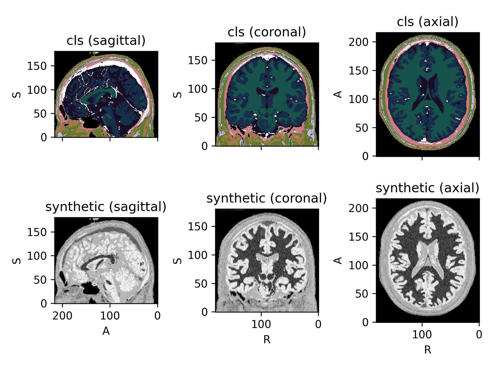
- class torchio.transforms.RandomLabelsToImage(label_key: str | None = None, used_labels: Sequence[int] | None = None, image_key: str = 'image_from_labels', mean: Sequence[float | Tuple[float, float]] | None = None, std: Sequence[float | Tuple[float, float]] | None = None, default_mean: float | Tuple[float, float] = (0.1, 0.9), default_std: float | Tuple[float, float] = (0.01, 0.1), discretize: bool = False, ignore_background: bool = False, **kwargs)[source]#
Bases:
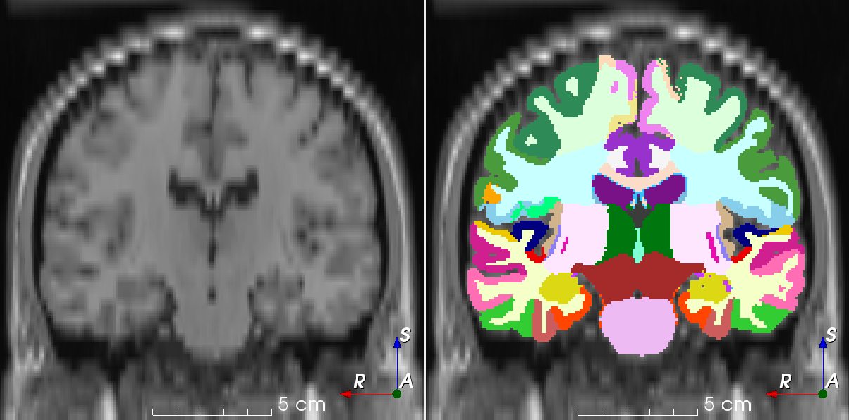
RandomTransform,IntensityTransformRandomly generate an image from a segmentation.
Based on the work by Billot et al.: A Learning Strategy for Contrast-agnostic MRI Segmentation and Partial Volume Segmentation of Brain MRI Scans of any Resolution and Contrast.
(
Source code,png)
- Parameters:
label_key – String designating the label map in the subject that will be used to generate the new image.
used_labels – Sequence of integers designating the labels used to generate the new image. If categorical encoding is used,
label_channelsrefers to the values of the categorical encoding. If one hot encoding or partial-volume label maps are used,label_channelsrefers to the channels of the label maps. Default uses all labels. Missing voxels will be filled with zero or with voxels from an already existing volume, seeimage_key.image_key – String designating the key to which the new volume will be saved. If this key corresponds to an already existing volume, missing voxels will be filled with the corresponding values in the original volume.
mean – Sequence of means for each label. For each value \(v\), if a tuple \((a, b)\) is provided then \(v \sim \mathcal{U}(a, b)\). If
None,default_meanrange will be used for every label. If notNoneandlabel_channelsis notNone,meanandlabel_channelsmust have the same length.std – Sequence of standard deviations for each label. For each value \(v\), if a tuple \((a, b)\) is provided then \(v \sim \mathcal{U}(a, b)\). If
None,default_stdrange will be used for every label. If notNoneandlabel_channelsis notNone,stdandlabel_channelsmust have the same length.default_mean – Default mean range.
default_std – Default standard deviation range.
discretize – If
True, partial-volume label maps will be discretized. Does not have any effects if not using partial-volume label maps. Discretization is done taking the class of the highest value per voxel in the different partial-volume label maps usingtorch.argmax()on the channel dimension (i.e. 0).ignore_background – If
True, input voxels labeled as0will not be modified.**kwargs – See
Transformfor additional keyword arguments.
Tip
It is recommended to blur the new images in order to simulate partial volume effects at the borders of the synthetic structures. See
RandomBlur.Example
>>> import torchio as tio
>>> subject = tio.datasets.ICBM2009CNonlinearSymmetric()
>>> # Using the default parameters
>>> transform = tio.RandomLabelsToImage(label_key='tissues')
>>> # Using custom mean and std
>>> transform = tio.RandomLabelsToImage(
...     label_key='tissues', mean=[0.33, 0.66, 1.], std=[0, 0, 0]
... )
>>> # Discretizing the partial volume maps and blurring the result
>>> simulation_transform = tio.RandomLabelsToImage(
...     label_key='tissues', mean=[0.33, 0.66, 1.], std=[0, 0, 0], discretize=True
... )
>>> blurring_transform = tio.RandomBlur(std=0.3)
>>> transform = tio.Compose([simulation_transform, blurring_transform])
>>> transformed = transform(subject)  # subject has a new key 'image_from_labels' with the simulated image
>>> # Filling holes of the simulated image with the original T1 image
>>> rescale_transform = tio.RescaleIntensity(
...     out_min_max=(0, 1), percentiles=(1, 99))   # Rescale intensity before filling holes
>>> simulation_transform = tio.RandomLabelsToImage(
...     label_key='tissues',
...     image_key='t1',
...     used_labels=[0, 1]
... )
>>> transform = tio.Compose([rescale_transform, simulation_transform])
>>> transformed = transform(subject)  # subject's key 't1' has been replaced with the simulated image
See also
RandomGamma#
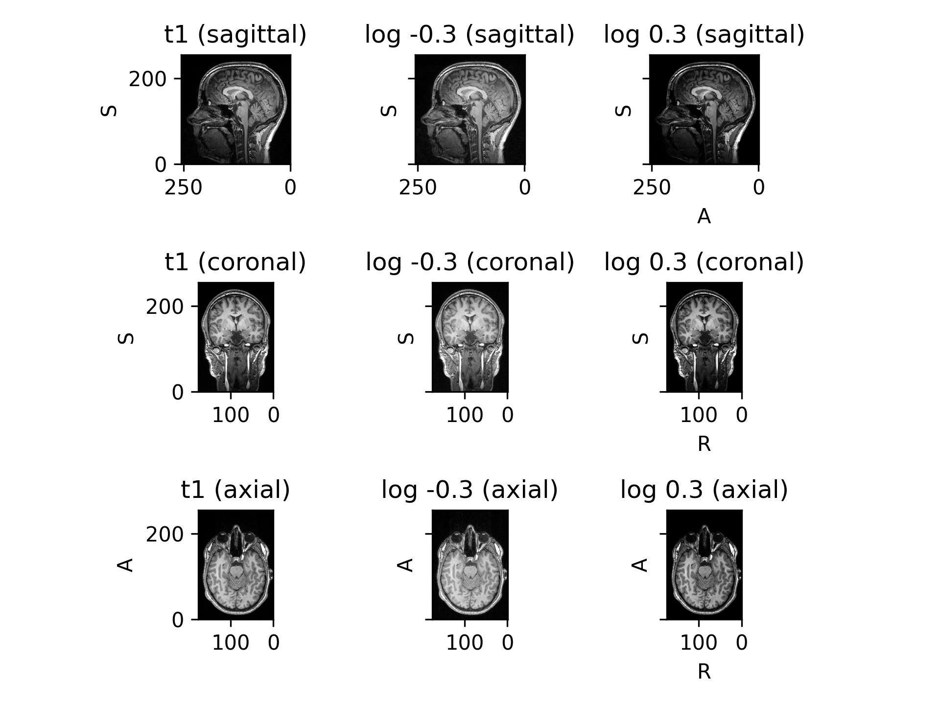
- class torchio.transforms.RandomGamma(log_gamma: float | Tuple[float, float] = (-0.3, 0.3), **kwargs)[source]#
Bases:
RandomTransform,IntensityTransformRandomly change contrast of an image by raising its values to the power \(\gamma\).
- Parameters:
log_gamma – Tuple \((a, b)\) to compute the exponent \(\gamma = e ^ \beta\), where \(\beta \sim \mathcal{U}(a, b)\). If a single value \(d\) is provided, then \(\beta \sim \mathcal{U}(-d, d)\). Negative and positive values for this argument perform gamma compression and expansion, respectively. See the Gamma correction Wikipedia entry for more information.
**kwargs – See
Transformfor additional keyword arguments.
Note
Fractional exponentiation of negative values is generally not well-defined for non-complex numbers. If negative values are found in the input image \(I\), the applied transform is \(\text{sign}(I) |I|^\gamma\), instead of the usual \(I^\gamma\). The
RescaleIntensitytransform may be used to ensure that all values are positive. This is generally not problematic, but it is recommended to visualize results on images with negative values. More information can be found on this StackExchange question.(
Source code,png)
Example
>>> import torchio as tio
>>> subject = tio.datasets.FPG()
>>> transform = tio.RandomGamma(log_gamma=(-0.3, 0.3))  # gamma between 0.74 and 1.34
>>> transformed = transform(subject)